 Database Tutorials MSSQL, Oracle, PostgreSQL, MySQL, MariaDB, DB2, Sybase, Teradata, Big Data, NOSQL, MongoDB, Couchbase, Cassandra, Windows, Linux
Teradata 15.0 has come up with many new exciting features and enhanced capabilities . Teradata Query Grid is one of them.
Teradata database now able to connect Hadoop with this Query Grid so it’s called as Teradata Database-to-Hadoop also referred as Teradata-to-Hadoop connector.
Key Importance of Teradata Query Grid is to Put Data in the Data Lake FAST across foreign servers.
What is Query Grid?
Query Grid works to connect a Teradata and Hadoop system to massive scale, with no effort, and at speeds of 10TB/second.
- It provides a SQL interface for transferring data between Teradata Database and remote Hadoop hosts.
- Import Hadoop data into a temporary or permanent Teradata table.
- Export data from temporary or permanent Teradata tables into existing Hadoop tables.
- Create or drop tables in Hadoop from Teradata Database.
- Reference tables on the remote hosts in SELECT and INSERT statements.
- Select Hadoop data for use with a business tool.
- Select and join Hadoop data with data from independent data warehouses for analytical use.
- Leverage Hadoop resources, Reduce data movement
- Bi-directional to Hadoop
- Query push-down
- Easy configuration of server connections
What could be the Process Flow ?
- Query through Teradata
- Sent to Hadoop through Hive
- Results returned to Teradata
- Additional processing joins data in Teradata
- Final results sent back to application/user
With QueryGrid, We can add a clause in a SQL statement that says
“Call up Hadoop, pass Hive a SQL request, receive the Hive results, and join it to the data warehouse tables.”
Running a single SQL statement spanning Hadoop and Teradata is amazing in itself a big deal within self. Notice too that all the database security, advanced SQL functions, and system management in the Teradata system is supporting these queries. The only effort required is for the database administrator to set up a “view” that connects the systems.
- QueryGrid
- Server grammar
- Simplify via “server name”
- Hadoop import operator
- Load_from_hcatalog
- Added server grammar
- Hadoop export operator (new)
- Load_to_hcatalog
- Supports files:
- Delimited Text, JSON, RCFile
- Sequence File, ORCfile, Avro
- Query push-down
- Bi-directional data transfer
- Provide access rights
Parallel Performance:
From many years, data virtualization tools lack the ability to move data between systems in parallel. Such tools send a request to a remote database and the data comes back serially through an Ethernet wire. Teradata Query Grid is built to link to remote systems in parallel and interchange data through many network connections at once.
If we want to move a terabyte per minute? With the right configurations it can be done. Parallel processing by both systems makes this extremely fast. I know of no data virtualization system that does this today.
Without doubt, the Hadoop cluster will have a different number of servers compared to the Teradata or any MPP systems. The Teradata systems start the parallel data exchange by matching up units of parallelism between the two systems. That is, all the Teradata parallel workers (called AMPs) connect to a buddy Hadoop worker node for maximum throughput. Anytime the configuration changes, the workers match-up changes.
But Teradata Query Grid does it all for us completely invisible to the user.
Query Grid Teradata to Hadoop Server Configuration:
CREATE FOREIGN SERVER Hadoop_sysd_xav USING HOSTTYPE(‘hadoop’)SERVER (‘sysd.labs.teradata.com’) PORT (‘9083’) HIVESERVER(‘sysd.labs.teradata.com’) HIVEPORT (‘10000’) USERNAME(‘Hive’)DEFAULT_STRING_SIZE(‘2048’)HADOOP_PROPERTIES(‘org.apache.hadoop.io.compress.GzipCodec’);
DO IMPORT WITH syslib.load_from_hcatalog_hdp1_3_2,
DO EXPORT WITH syslib.load_to_hcatalog_hdp1_3_2Merge_hdfs_files(‘True’)Compression_codec(‘org.apache.hadoop.io.compress.GzipCodec’;
Server name = Hadoop_sysd_xav
Table Name = xav_hdp_tbl@Hadoop_sysd_xav
SELECT source, session
FROM xav_hdp_tbl@Hadoop_sysd_xav
WHERE session_ts = ‘2017-01-01’;
QueryGrid Server Objects and Privileges:
1) TD_SERVER_DB contains all servers objects
2) Servers are global objects
3) Users have SELECT and INSERT granted to them
- a) GRANT SELECT ON hdp132_svr TO Pankaj;
- b) GRANT INSERT ON hdp143_svr TO Abid;
4) Being able to create and drop a server is a privilege
- a) GRANT CREATE SERVER
- b) GRANT DROP SERVER
Remote SQL Execution :
1) Push SQL to remote Hive system
2) Hive filters data on non-partitioned columns
3) Foreign table ‘Select’ executed on remote system
SELECT source, session
FROM FOREIGN TABLE(
select session, source
from xav_hdp_tbl
where source = “Mozilla” )@Hadoop_sysd_xav
WHERE session = current_date AS dt;
QueryGrid Data Transfer:
Import
SELECT source, session
FROM xav_hdp_tbl@Hadoop_sysd_xav
WHERE session_ts = ‘2017-01-01’; “insert/select” & “create table as” to instantiate data locally.
Export
INSERT INTO emp_xav@Hadoop_sysd_xav
SELECT emp_xav_id, emp_xav_zip
FROM emp_xav_data
WHERE last_update = current_date;
QueryGrid Insert Explained :
EXPLAIN INSERT INTO xav_data@hdp132_svr SELECT * FROM newcars;
***Success: Activity Count = 41 Explanation —————————————————————————
1) First, we lock a distinct ut1.”pseudo table” for read on a RowHash to prevent global deadlock for ut1.tab1.
2) Next, we lock ut1.tab1 for read.
3) We do an all-AMPs RETRIEVE step from ut1.newcars by way of an all–rows scan with no residual conditions executing table operator SYSLIB.load_to_hcatalog with a condition of (“(1=1)”) into Spool 2 (used to materialize view, derived table, table function or table operator drvtab_inner) (all_amps), which is built locally on the AMPs. The size of Spool 2 is estimated with low confidence to be 8 rows (11,104 bytes). The estimated time for this step is 0.16 seconds.
4) We do an all-AMPs RETRIEVE step from Spool 2 (Last Use) by way of an all–rows scan into Spool 3 (used to materialize view, derived table, table function or table operator TblOpInputSpool) (all_amps), which is redistributed by hash code to all AMPs. The size of Spool 3 is estimated with low confidence to be 8 rows ( 11,104 bytes). The estimated time for this step is 0.16 seconds.
5) We do an all-AMPs RETRIEVE step from Spool 3 (Last Use) by way of an all–rows scan executing table operator SYSLIB.load_to_hcatalog with a condition of (“(1=1)”) into Spool 4 (used to materialize view, derived table, table function or table operator h4) (all_amps), which is built locally on the AMPs.
< BEGIN EXPLAIN FOR REMOTE QUERY –> TD: 3 column(s); Hadoop: 3 column(s), with 2 partition column(s); doors(INTEGER) -> doors(STRING); make(VARCHAR) -> make*(STRING); model(VARCHAR) -> model*(STRING); * denotes partition column;
<— END EXPLAIN FOR REMOTE QUERY > The size of Spool 4 is estimated with low confidence to be 8 rows (200 bytes). The estimated time for this step is 0.16 seconds.
Create and Drop Hadoop Tables:
1) Stored procedures to create and drop Hadoop tables
2) Allows SQL scripts to export data in stand alone fashion
CALL SYSLIB.HDROP(‘t3′,’hdp132_svr’);
CALL SYSLIB.HCTAS(‘t3′,’c2,c3’,’LOCATION “/user/hive/table_t12″‘,’hdp132_svr’,’default’);
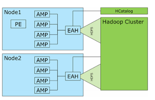
Connection Flow:
- The client connects to the system through the PE in node 1. The query is parsed in the PE. During the parsing phase, the table operator’s contract function contacts the HCatalog component through the External Access Handler (EAH), which is a one-per-node Java Virtual Machine Connection Flow
- The HCatalog returns the metadata about the table, the number of columns, and the types for the columns. The parser uses this info and also uses this connection d to obtain the Hadoop splits of data that underlie the Hadoop table.
- The splits are assigned to the AMPs in a round-robin fashion so that each AMP gets a split.
- The parser phase completes and produces an AMP step containing the table operator. This is sent to all the AMPs in parallel.
- Each AMP then begins to execute the table operator’s execute function providing a parallel import of Hadoop data.
- The execute function opens and reads the split data reading in Hadoop rows. These are converted to Teradata data types in each column, and the rows are written to spool.
- When all the data has been written, the spool file is redistributed as input into the next part of the query plan.
Performance/Speed:
Imagine complex systematic analytics using R or SAS are run inside the Teradata data warehouse as part of a merger and acquisition project. In this case, we want to pass this data to the Hadoop Data Lake where it is combined with temporary data from the company being acquired. With reasonably simple SQL stuffed in a database view, the answers calculated by the Teradata Database can be sent to Hadoop to help finish up some reports. Bi-directional data exchange is another breakthrough in the Teradata Query Grid, new in release 15.0. The common thread in all these innovations is that the data moves from the memory of one system to the memory of the other. No extracts, no landing the data on disk until the final processing step – and sometimes not even then.
What is Push-down Processing:
To minimize data movement, Teradata Query Grid sends the remote system SQL filters that eliminate records and columns that aren’t needed.
This way, the Hadoop system discards unnecessary data so it doesn’t flood the network with data that will be thrown away. After all the processing is done in Hadoop, data is joined in the data warehouse, summarized, and delivered to the user’s favorite business intelligence tool.
Business Benefits:
- No hassle analytics with a seamless data fabric across all of our data and analytical engines
- Get the most out of your data by taking advantage of specialized processing engines operating as a cohesive analytic environment
- Transparently harness the combined power of multiple analytic engines to address a business question
- Self-service data and analytics across all systems through SQL
IT Benefits
- Automate and optimize use of your analytic systems through “push-down” processing across platforms
- Minimize data movement and process data where it resides
- Minimize data duplication
- Transparently automate analytic processing and data movement between systems
- Enable easy bi-directional data movement
- Integrated processing without administrative challenges
- Leverage the analytic power and value of your Teradata Database, Teradata Aster Database, open-source Presto and Hive for Hadoop, Oracle Database, and powerful languages such as SAS, Perl, Python, Ruby, and R.
- High performance query plans using data from other sources while using systems within the Teradata Unified Data Architecture such as passing workload priorities makes the best use of available resources
Requirements for Query Grid to Hadoop:
1) Teradata 15.0 +
2) Node memory > 96GB
- a)Network > All Teradata nodes able to connect to all Hadoop data nodes
- b)Proxy user on Hadoop
References:
http://www.teradata.com
https://en.wikipedia.org
http://in.teradata.com/products-and-services/query-grid/?LangType=16393&LangSelect=true
http://www.info.teradata.com/download.cfm?ItemID=1001944
![]()